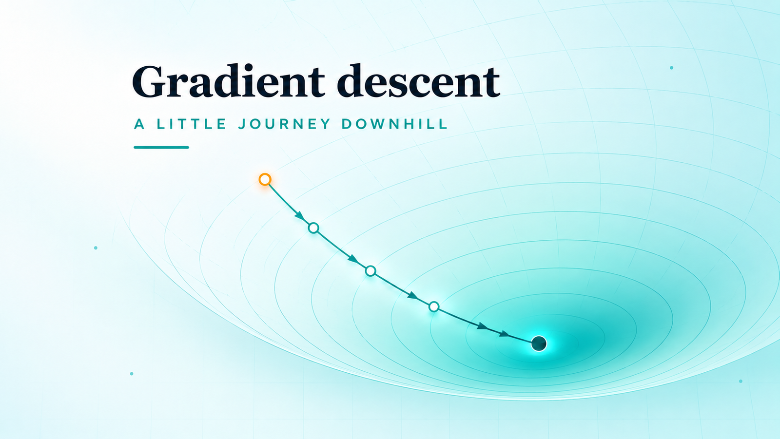
Machine learning · A worked visual guide
Gradient descent:
finding the way down.
I want to understand how a model improves, not just memorize an equation. So I’ll start with five observations, build a line that predicts them, measure how wrong it is, and update that line one careful step at a time.
01 / Start with actual data
What line are we trying to learn?
Imagine I collected five observations. Each one records how many hours a student studied and the score they received. The points do not sit perfectly on one line, so I need a model that captures the overall pattern rather than passing through every point.
| Observation | Study hours | Observed score |
|---|---|---|
| 1 | 1 | 35 |
| 2 | 2 | 42 |
| 3 | 3 | 55 |
| 4 | 4 | 61 |
| 5 | 5 | 72 |
For each study-hour value, the model produces a prediction. I’ll use a straight-line model with two adjustable parameters:
To keep the numbers easy to work with, I centre and scale study hours:
So the five input values become −1, −0.5, 0, 0.5, 1. In this version of the model, b is the predicted score at 3 study hours, and m is how much the prediction changes when study time increases by 2 hours. This is still an ordinary straight line; centring the input just makes the arithmetic cleaner.
I’ll begin with a deliberately poor guess: b = 20 and m = 5. That gives a low, fairly flat line. The model is underpredicting every observation.
| Hours | Scaled x | Actual y | Initial prediction | Error (prediction − actual) |
|---|---|---|---|---|
| 1 | −1 | 35 | 15 | −20 |
| 2 | −0.5 | 42 | 17.5 | −24.5 |
| 3 | 0 | 55 | 20 | −35 |
| 4 | 0.5 | 61 | 22.5 | −38.5 |
| 5 | 1 | 72 | 25 | −47 |
Important: these five values are a small teaching dataset, not evidence that studying a particular number of hours causes a particular score. We are using them to understand the optimization mechanics.
02 / Give “wrong” a number
How do I measure whether the line is bad?
Looking at a graph is useful, but an algorithm needs a numerical score. I’ll compare every prediction with its observed score, square each error so positive and negative errors do not cancel, and average the result.
Here n = 5, and the prediction for observation i is b + m xᵢ. The factor of 1/2 is included because it cancels the 2 that appears when we differentiate a squared error. It does not change which parameters give the smallest loss.
For my starting line, the errors are −20, −24.5, −35, −38.5 and −47. Squaring and adding them gives:
That number is our starting point. Gradient descent does not know what a “good-looking line” is. It only knows the loss function I gave it, and it tries to make that number smaller.
03 / Find the direction
What does the gradient actually tell me?
The loss depends on two parameters, b and m. So there are two questions: what happens to the loss if I nudge b, and what happens if I nudge m? Those two rates of change make the gradient.
Write the error for one observation as eᵢ = b + m xᵢ − yᵢ. Our loss is the average of the squared errors, with the factor of 1/2:
Differentiate with respect to b. The derivative of eᵢ with respect to b is 1, so the 2 from the square cancels the 1/2:
Now differentiate with respect to m. Because m is multiplied by xᵢ, the derivative of eᵢ with respect to m is xᵢ:
At the starting guess, the errors are the five values from the table and the scaled inputs are −1, −0.5, 0, 0.5, 1. Therefore:
So the gradient is (−33, −6.8). It points in the direction where the loss increases fastest. Both components are negative, which tells me that increasing b and increasing m will reduce the loss from this starting point. The downhill direction is the opposite of the gradient.
04 / Make one real update
Turn the gradient into a better line
The learning rate, usually written as α (alpha), controls how much of the gradient I follow. I’ll choose α = 0.2 for this first worked step.
Update b and m using the gradients we just calculated. Both updates use the same old parameter values; they happen together, not one after the other.
Now the model is prediction = 26.6 + 6.36x. Its predictions are 20.24, 23.42, 26.6, 29.78 and 32.96. The new loss is 386.8444, down from 591.65. One update has made the line better according to our chosen loss function.
Notice what happened: we did not tell the model “raise the line by 6.6” or “make the slope 6.36”. The gradients and learning rate calculated those changes from the data.
05 / Repeat, don't guess
What happens over several updates?
Every step repeats the same routine: calculate predictions, calculate errors, calculate both gradients, update both parameters, and measure the new loss. With α = 0.2, the first few updates are:
| Step | b | m | Loss |
|---|---|---|---|
| 0 · Start | 20.000 | 5.000 | 591.650 |
| 1 | 26.600 | 6.360 | 386.844 |
| 2 | 31.880 | 7.584 | 254.275 |
| 3 | 36.104 | 8.686 | 168.221 |
| 4 | 39.483 | 9.677 | 112.167 |
| 5 | 42.187 | 10.569 | 75.498 |
The values in this table are calculated from the same five observations and the same gradient formulas shown above. The interactive lab below runs these actual updates; it does not move along a precomputed path to the answer.
06 / Now make the idea visible
Watch both parameters learn
The left plot shows the loss landscape over the two parameters b and m. Each contour is a set of parameter pairs with the same loss. The right plot shows the line those parameters produce against the five observations. When I take a step, both views update from the same calculation.
1. Loss landscape · L(b,m)Click to choose b and m
The dot is the current parameter pair. Contours closer to the centre have lower loss. The teal arrow shows the negative-gradient direction: the way to step downhill.
2. Prediction line · data fitb = 20.0 · m = 5.0
Teal dots are the observations. The orange line is the model's current prediction. Dashed vertical gaps are prediction errors.
| Step | b | m | Loss |
|---|---|---|---|
| 0 | 20.000 | 5.000 | 591.650 |
The contour plot is calculated from the same loss function as the line plot. It is not a decorative valley or a separate animation: each point represents a real pair of model parameters.
07 / Why the learning rate matters
Why not take the biggest step possible?
The gradient tells me which way is downhill, but the learning rate decides how far I move in that direction. A direction can be correct while the step is too large.
Too small: the updates reduce the loss, but progress is slow. I may need many iterations.
Reasonable: the loss falls steadily and the parameter pair approaches the minimum.
Too large: an update can cross the bottom of the valley. It may bounce from one side to the other. If it is large enough, the loss increases and the process diverges.
Because we centred and scaled x, the two curvature values for this particular loss surface are 1 and 0.5. That makes a constant learning rate between 0 and 2 stable for this example. Near 2, one parameter direction can oscillate strongly. At exactly 2, the b update does not shrink; above 2, it diverges. This threshold is specific to this model and scaling—not a universal learning-rate rule.
08 / Put the steps into code
The algorithm is a small loop
This Python code performs exactly the calculation used by the interactive lab. It uses every observation to calculate each gradient, so this is batch gradient descent.
import numpy as np

hours = np.array([1, 2, 3, 4, 5], dtype=float)
y = np.array([35, 42, 55, 61, 72], dtype=float)

# Centre and scale the input: [-1, -0.5, 0, 0.5, 1]
x = (hours - 3) / 2

b = 20.0
m = 5.0
learning_rate = 0.20

for step in range(100):
    predictions = b + m * x
    errors = predictions - y

    loss = np.mean(errors ** 2) / 2
    db = np.mean(errors)
    dm = np.mean(errors * x)

    # Both updates use gradients from the same old parameters.
    b = b - learning_rate * db
    m = m - learning_rate * dm

print("b:", b)
print("m:", m)
The order matters: first calculate both gradients from the current predictions, then update both parameters. If I update b before calculating the gradient for m, I would accidentally mix two different parameter states.
09 / Know what the result means
Where does the algorithm end up?
For these five observations, the minimum-loss line is approximately b = 53 and m = 18.6. Remember what those parameters mean: 53 is the predicted score at 3 study hours, and 18.6 is the predicted change across 2 additional study hours.
In the original, unscaled study-hours variable, this same line is approximately score = 25.1 + 9.3 × hours. The minimum loss is about 0.91, not zero. That is expected: the five observations do not lie perfectly on a straight line. The goal is not to force every point onto the line; it is to find the parameters that minimize the chosen squared-error loss.
This example is linear regression, whose squared-error loss is a convex bowl with one global minimum. Neural networks can have much more complicated loss surfaces, but the central operation is the same: calculate a gradient and adjust parameters in the negative-gradient direction.
One final caution: reducing training loss only means the model fits these five examples better. It does not prove that study hours cause higher scores or that the model will predict new students accurately. For that, we would need more data and a separate test set.
10 / Continue learning
Good next explanations
These are worth opening after working through the numbers above. The first develops the mathematical treatment; the second builds a visual intuition for gradient descent in machine learning.
- Stanford CS229 · Supervised Learning and Gradient DescentLecture notes with the cost function, gradient update and batch gradient descent.
- 3Blue1Brown · Gradient descent, how neural networks learnA visual explanation of loss, gradients and parameter updates.
- scikit-learn · LinearRegressionReference for ordinary least-squares linear regression and its fitted coefficients.